How To Use Conditional Formatting In Excel To Change Cell Color - In microsoft excel 2010, i'm trying to apply a fill color to a cell based on the value in an adjacent cell.

How To Use Conditional Formatting In Excel To Change Cell Color - In microsoft excel 2010, i'm trying to apply a fill color to a cell based on the value in an adjacent cell.. =countif($ah$4:$ah$16,b$5)>1 then, in the dialog box manage rules, select the range b4:af11. Note:in this case, you must lock the reference of the row so that the conditional format will work correctly in the other cells in this table. =weekday(b$5,2)>5 the parameter 2 means saturday = 6 and sunday = 7. Scale = 3 colors 1.2. In the text box format values where this formula is true,enter the following weekday formula to determine whether the cell is a saturday (6) or sunday (7):

How to automatically color code in excel? =countif($ah$4:$ah$16,b$5)>1 then, in the dialog box manage rules, select the range b4:af11. Purple dates more than 3 months we then construct three rules conditional formatting using formula datedif. respectively for the three cases the following formulas: You can select the following date options, ranging from yesterday to next month: Scale = 3 colors 1.2.

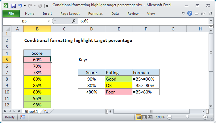
Excel formula: Conditional formatting highlight target ... from exceljet.net

See full list on microsoft.com In the following example, we show: You can select the following date options, ranging from yesterday to next month: Minimum = 0 red 1.3. Purple dates more than 3 months we then construct three rules conditional formatting using formula datedif. respectively for the three cases the following formulas: Change the value of the month and the year to see how the calendar has a different format. In the text box format values where this formula is true,enter the following weekday formula to determine whether the cell is a saturday (6) or sunday (7): In this case, we use the formula countifin order to count if the number of public holidays in the current month is greater than 1.

In the new formatting rule dialog, click use a formula to determine which cells to format in select a rule type section, and type =$c1>$g$2 into the format values where this formula is true.

This example in the excel web app below shows the result. In microsoft excel 2010, i'm trying to apply a fill color to a cell based on the value in an adjacent cell. If you need to create rules for other dates (e.g., greater than a month from the current date), you can create your own new rule. =weekday(b$5,2)>5 the parameter 2 means saturday = 6 and sunday = 7. If you want to highlight the holidays over the weekends, you move the public holiday rule to the top of the list. See full list on microsoft.com What is a conditional formula in excel? Midpoint = 10 yellow 1.4. Now select use a formula to determine which cells to format option, and in the box type the formula: See full list on microsoft.com Again, open the menu conditional formatting > new rule. Change the value of the month and the year to see how the calendar has a different format. Yellow dates between 1 and 2 months 2.

Maximum = 30 white the result is a gradient color scale with nuances from white to red through yellow. To change the color of the weekends, open the menu conditional formatting > new rule in the next dialog box, select the menu use a formula to determine which cell to format. You can select the following date options, ranging from yesterday to next month: To find conditional formatting for dates, go to home > conditional formatting > highlight cell rules > a date occuring. In the following example, we show:

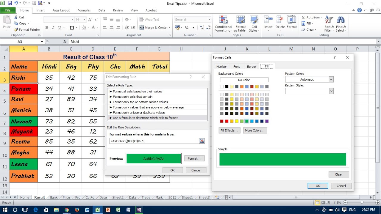
COURSES: How to do the Conditional Formatting in MS Excel from 1.bp.blogspot.com

When you design an automated calendar you don't need to color the weekends yourself. with the conditional formatting tool, you can automatically change the colors of weekends by basing the format on the weekday function. =weekday(b$5,2)>5 the parameter 2 means saturday = 6 and sunday = 7. This parameter is very useful to test for weekends. In the ribbon, select home > conditional formatting > new rule. See full list on microsoft.com If you want to highlight the holidays over the weekends, you move the public holiday rule to the top of the list. See full list on microsoft.com Then select format button to select green as the fill color.

What is a conditional formula in excel?

Note:in this case, you must lock the reference of the row so that the conditional format will work correctly in the other cells in this table. Again, open the menu conditional formatting > new rule. To change the color of the weekends, open the menu conditional formatting > new rule in the next dialog box, select the menu use a formula to determine which cell to format. Select "use a formula to determine which cells to format", and enter the following formula: Now select use a formula to determine which cells to format option, and in the box type the formula: In case we want to change the color of cells based on our approach on a date again, we will use conditional formatting to make it work for us. Midpoint = 10 yellow 1.4. Then select format button to select green as the fill color. Make sure the cell on which you want to apply conditional formatting is selected now select use a formula to determine which cells to format, and in the box use the formula, d3>5, then select the formatting to fill the cell color to green. See full list on microsoft.com Scale = 3 colors 1.2. In this case, we use the formula countifin order to count if the number of public holidays in the current month is greater than 1. How do you make cell color in excel?

See full list on microsoft.com Again, open the menu conditional formatting > new rule. See full list on microsoft.com In microsoft excel 2010, i'm trying to apply a fill color to a cell based on the value in an adjacent cell. Midpoint = 10 yellow 1.4.

Use a Formula in Conditional Formatting - Excel - YouTube from i.ytimg.com

Minimum = 0 red 1.3. =countif($ah$4:$ah$16,b$5)>1 then, in the dialog box manage rules, select the range b4:af11. Click apply to apply the formatting to your selected range and then click close. Orange dates between 2 and 3 months 3. Change the value of the month and the year to see how the calendar has a different format. Note:in this case, you must lock the reference of the row so that the conditional format will work correctly in the other cells in this table. Jun 27, 2021 · then click the format… button to choose what background color to apply when the above condition is met. Then select format button to select green as the fill color.

Yellow dates between 1 and 2 months 2.

In the new formatting rule dialog, click use a formula to determine which cells to format in select a rule type section, and type =$c1>$g$2 into the format values where this formula is true. Click format button to open format cells dialog, under font tab, select a font color you use. Jun 27, 2021 · then click the format… button to choose what background color to apply when the above condition is met. Make sure the cell on which you want to apply conditional formatting is selected now select use a formula to determine which cells to format, and in the box use the formula, d3>5, then select the formatting to fill the cell color to green. See full list on microsoft.com How to automatically color code in excel? If you need to create rules for other dates (e.g., greater than a month from the current date), you can create your own new rule. Maximum = 30 white the result is a gradient color scale with nuances from white to red through yellow. See full list on microsoft.com To find conditional formatting for dates, go to home > conditional formatting > highlight cell rules > a date occuring. Now select use a formula to determine which cells to format option, and in the box type the formula: See full list on microsoft.com =e4="overdue" click on the format button and select your desired formatting.

Then select format button to select green as the fill color how to use conditional formatting in excel. When you design an automated calendar you don't need to color the weekends yourself. with the conditional formatting tool, you can automatically change the colors of weekends by basing the format on the weekday function.

Source: i.ytimg.com

Jun 27, 2021 · then click the format… button to choose what background color to apply when the above condition is met. In the ribbon, select home > conditional formatting > new rule. These 10 date options generate rules based on the current date. To find conditional formatting for dates, go to home > conditional formatting > highlight cell rules > a date occuring. Again, open the menu conditional formatting > new rule.

Source: www.wikihow.com

Maximum = 30 white the result is a gradient color scale with nuances from white to red through yellow. First, go into a new column (column e), calculate the difference in number of days in a year again with the datedif formula and the parameter "yd". Select "use a formula to determine which cells to format", and enter the following formula: Click format button to open format cells dialog, under font tab, select a font color you use. See full list on microsoft.com

Source: heelpbook.altervista.org

These 10 date options generate rules based on the current date. This example in the excel web app below shows the result. Click apply to apply the formatting to your selected range and then click close. Minimum = 0 red 1.3. In the format cells dialog box, switch to the fill tab and select the color of your choice, the reddish color in our case, and click ok.

Source: www.exceltip.com

=datedif($d2,today(),"yd") then choose the menu conditional formatting> new ruleoption format all cells based on their value and choose the following options: See full list on microsoft.com First, go into a new column (column e), calculate the difference in number of days in a year again with the datedif formula and the parameter "yd". Jun 27, 2021 · then click the format… button to choose what background color to apply when the above condition is met. =weekday(b$5,2)>5 the parameter 2 means saturday = 6 and sunday = 7.

Source: support.content.office.net

Note:in this case, you must lock the reference of the row so that the conditional format will work correctly in the other cells in this table. In the text box format values where this formula is true,enter the following weekday formula to determine whether the cell is a saturday (6) or sunday (7): To do that, you need a column with the holidays you'd like to highlight in your workbook (but not necessarily in the same sheet). in our example, we have us public holidays in column ah (as related to the year in the cell b2). Again, open the menu conditional formatting > new rule. How to automatically color code in excel?

Source: www.meadinkent.co.uk

Midpoint = 10 yellow 1.4. On the home tab, in the styles subgroup, click on conditional formatting→new rule. Now select use a formula to determine which cells to format option, and in the box type the formula: Maximum = 30 white the result is a gradient color scale with nuances from white to red through yellow. You can select the following date options, ranging from yesterday to next month:

Source: www.extendoffice.com

In the format cells dialog box, switch to the fill tab and select the color of your choice, the reddish color in our case, and click ok. See full list on microsoft.com =datedif($b2,$e$2,"m")>0 =datedif($b2,$e$2,"m")>1 =datedif($b2,$e$2,"m")>2 in the excel web app below, try changing some dates to experiment with the result. Midpoint = 10 yellow 1.4. Click format button to open format cells dialog, under font tab, select a font color you use.

Source: i.ytimg.com

These 10 date options generate rules based on the current date. In microsoft excel 2010, i'm trying to apply a fill color to a cell based on the value in an adjacent cell. Midpoint = 10 yellow 1.4. How do you make cell color in excel? Now select use a formula to determine which cells to format option, and in the box type the formula:

Source: www.wikihow.com

Select "use a formula to determine which cells to format", and enter the following formula: =weekday(b$5,2)>5 the parameter 2 means saturday = 6 and sunday = 7. In this case, we use the formula countifin order to count if the number of public holidays in the current month is greater than 1. In the following example, we show: =datedif($b2,$e$2,"m")>0 =datedif($b2,$e$2,"m")>1 =datedif($b2,$e$2,"m")>2 in the excel web app below, try changing some dates to experiment with the result.

Source: www.exceldemy.com

This parameter is very useful to test for weekends.

Source: www.techonthenet.com

Click apply to apply the formatting to your selected range and then click close.

Source: www.librt.com

What is a conditional formula in excel?

Source: support.content.office.net

Jun 27, 2021 · then click the format… button to choose what background color to apply when the above condition is met.

Source: i.ytimg.com

In the format cells dialog box, switch to the fill tab and select the color of your choice, the reddish color in our case, and click ok.

Source: searchengineland.com

To find conditional formatting for dates, go to home > conditional formatting > highlight cell rules > a date occuring.

Source: filestore.community.support.microsoft.com

If you want to highlight the holidays over the weekends, you move the public holiday rule to the top of the list.

Source: cdn.ablebits.com

Yellow dates between 1 and 2 months 2.

Source: d2myx53yhj7u4b.cloudfront.net

In the new formatting rule dialog, click use a formula to determine which cells to format in select a rule type section, and type =$c1>$g$2 into the format values where this formula is true.

Source: cdn.ablebits.com

Then, customize the format of your condition by clicking on the formatbutton and you choose a fill colo.

Source: cdn.e-iceblue.com

In microsoft excel 2010, i'm trying to apply a fill color to a cell based on the value in an adjacent cell.

Source: exceljet.net

In the format cells dialog box, switch to the fill tab and select the color of your choice, the reddish color in our case, and click ok.

Source: cdn.extendoffice.com

In the ribbon, select home > conditional formatting > new rule.

Source: infojinx.com

See full list on microsoft.com

Source: www.easyclickacademy.com

Then select format button to select green as the fill color.

Source: spreadsheeto.com

Make sure the cell on which you want to apply conditional formatting is selected now select use a formula to determine which cells to format, and in the box use the formula, d3>5, then select the formatting to fill the cell color to green.

Source: www.howtogeek.com

Then, customize the format of your condition by clicking on the formatbutton and you choose a fill colo.

Source: www.easyclickacademy.com

To do that, you need a column with the holidays you'd like to highlight in your workbook (but not necessarily in the same sheet). in our example, we have us public holidays in column ah (as related to the year in the cell b2).

Share :